Will the customer buy product after the haircut?
This will be based off the survey data we have of over 100 responses
The Dataset
The following features from the survey are measured and included within the CSV:
- Timestamp
- E-mail Address
- Work Zip Code
- Home Zip Code
- Business Name
- City, State last haircut
- Gender
- Age
- Race
- Income Range
- Time since last haircut
- Time between haircuts
- Buy Products
- How much spent last haircut
- Maximum spend for haircut
- How find current barber
- Leave reviews online
- Importance of Price (1-5)
- Importance of Convenience (1-5)
- Importance of Atmosphere (1-5)
- Importance of Additional Services (1-5)
- Additional Comments
Correlation Matrix

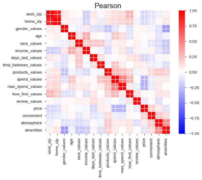
From the pearson correlation matrix populated from pandas_profiling, we can see the fields that have a strong correlation to the 'Buy Products' response.
We will import the numeric_survey csv output from the latest survey and create a new dataframe with just the fields with strong correlations
#import dependencies
%matplotlib inline
import matplotlib.pyplot as plt
import pandas as pd
import numpy as np

from sklearn.metrics import accuracy_score
# read in CSV from numeric_survey function
df = pd.read_csv('../data/survey04172018.csv',index_col=None)
df.head()
# create new dataframe with fields from correlation matrix
df2 = df[['products_values','spend_values','max_spend_values','atmosphere','amenities']]
df2.head()
# sum of 'Buy Product' responses
df2.products_values.sum()
Taking the sum of the product values we can see that from our survey we will have an imbalanced class. Over 80% of the answers from the survey were 'No'.
To account for this discrepany we will Up-sample the minority class
Up-sampling is the process of randomly duplicating observations from the minority class in order to reinforce its signal.
https://elitedatascience.com/imbalanced-classes
Up-sampling the minority class
# import dependency from sklearn to resample
from sklearn.utils import resample
# Separate majority and minority classes
df_majority = df2[df2.products_values==0]
df_minority = df2[df2.products_values==1]

# Upsample minority class
df_minority_upsampled = resample(df_minority,
                                 replace=True,     # sample with replacement
                                 n_samples=104,    # to match majority class
                                 random_state=17) # reproducible results

# Combine majority class with upsampled minority class
df_upsampled = pd.concat([df_majority, df_minority_upsampled])

# Display new class counts
df_upsampled.products_values.value_counts()
Split our data into training and testing.
# Assign X (data) and y (target)
y = df_upsampled.products_values
X = df_upsampled.drop('products_values', axis=1)

print(X.shape, y.shape)
# split sample into training and test
from sklearn.model_selection import train_test_split

X_train, X_test, y_train, y_test = train_test_split(X, y, random_state=1, stratify=y)
Create a Logistic Regression Model
### set class_weight to balanced
from sklearn.linear_model import LogisticRegression
classifier = LogisticRegression(class_weight='balanced')
classifier
Fit (train) or model using the training data
### BEGIN SOLUTION
classifier.fit(X_train, y_train)
### END SOLUTION
Validate the model using the test data
### BEGIN SOLUTION
print(f"Training Data Score: {classifier.score(X_train, y_train)}")
print(f"Testing Data Score: {classifier.score(X_test, y_test)}")
### END SOLUTION
From the training data we currently have a data score of 0.79 and test data score of 0.52.
Ideally we would have wanted to have more survey results to create pull from a larger sampling. This was just a start and something we can build on with more responses.
Make predictions
# predict using x_test sample
predictions = classifier.predict(X_test)
print(f"First 10 Predictions:   {predictions[:10]}")
print(f"First 10 Actual labels: {y_test[:10].tolist()}")
# create data frame to show results
pd.DataFrame({"Prediction": predictions, "Actual": y_test}).reset_index(drop=True)